- Limitations of the Least Square Method
What is the Least Square Method?
Least Square Method is used to derive a generalized linear equation between two variables. when the value of the dependent and independent variable is represented as the x and y coordinates in a 2D cartesian coordinate system. Initially, known values are marked on a plot. The plot obtained at this point is called a scatter plot.
Then, we try to represent all the marked points as a straight line or a linear equation . The equation of such a line is obtained with the help of the Least Square method. This is done to get the value of the dependent variable for an independent variable for which the value was initially unknown. This helps us to make predictions for the value of dependent variable.
Least Square Method Definition
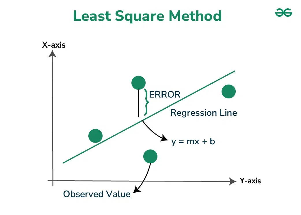
Least Squares method is a statistical technique used to find the equation of best-fitting curve or line to a set of data points by minimizing the sum of the squared differences between the observed values and the values predicted by the model.
This method aims at minimizing the sum of squares of deviations as much as possible. The line obtained from such a method is called a regression line or line of best fit .
Formula for Least Square Method
Least Square Method formula is used to find the best-fitting line through a set of data points. For a simple linear regression, which is a line of the form y =m x + c , where y is the dependent variable, x is the independent variable, a is the slope of the line, and b is the y-intercept, the formulas to calculate the slope ( m ) and intercept ( c ) of the line are derived from the following equations:
- n is the number of data points,
- ∑ xy is the sum of the product of each pair of x and y values,
- ∑ x is the sum of all x values,
- ∑ y is the sum of all y values,
- ∑ x 2 is the sum of the squares of x values.
The steps to find the line of best fit by using the least square method is discussed below:
- Step 1: Denote the independent variable values as x i and the dependent ones as y i .
- Step 2: Calculate the average values of x i and y i as X and Y.
- Step 3: Presume the equation of the line of best fit as y = mx + c, where m is the slope of the line and c represents the intercept of the line on the Y-axis.
- Step 4: The slope m can be calculated from the following formula:
- Step 5: The intercept c is calculated from the following formula:
Thus, we obtain the line of best fit as y = mx + c, where values of m and c can be calculated from the formulae defined above.
These formulas are used to calculate the parameters of the line that best fits the data according to the criterion of the least squares, minimizing the sum of the squared differences between the observed values and the values predicted by the linear model.
Least Square Method Graph
Let us have a look at how the data points and the line of best fit obtained from the Least Square method look when plotted on a graph.
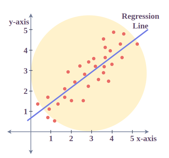
The red points in the above plot represent the data points for the sample data available. Independent variables are plotted as x-coordinates and dependent ones are plotted as y-coordinates . The equation of the line of best fit obtained from the Least Square method is plotted as the red line in the graph.
We can conclude from the above graph that how the Least Square method helps us to find a line that best fits the given data points and hence can be used to make further predictions about the value of the dependent variable where it is not known initially.
Limitations of the Least Square Method
The Least Square method assumes that the data is evenly distributed and doesn’t contain any outliers for deriving a line of best fit. But, this method doesn’t provide accurate results for unevenly distributed data or for data containing outliers.
Least Square Method Solved Examples
Problem 1: Find the line of best fit for the following data points using the Least Square method: (x,y) = (1,3), (2,4), (4,8), (6,10), (8,15).
Solution:
Here, we have x as the independent variable and y as the dependent variable. First, we calculate the means of x and y values denoted by X and Y respectively.
X = (1+2+4+6+8)/5 = 4.2
Y = (3+4+8+10+15)/5 = 8
| x i | y i | X – x i | Y – y i | (X-x i )*(Y-y i ) | (X – x i ) 2 |
|---|---|---|---|---|---|
| 1 | 3 | 3.2 | 5 | 16 | 10.24 |
| 2 | 4 | 2.2 | 4 | 8.8 | 4.84 |
| 4 | 8 | 0.2 | 0 | 0 | 0.04 |
| 6 | 10 | -1.8 | -2 | 3.6 | 3.24 |
| 8 | 15 | -3.8 | -7 | 26.6 | 14.44 |
| Sum (Σ) | 0 | 0 | 55 | 32.8 |
The slope of the line of best fit can be calculated from the formula as follows:
m = (Σ (X – x i )*(Y – y i )) /Σ(X – x i ) 2
m = 55/32.8 = 1.68 (rounded upto 2 decimal places)
Now, the intercept will be calculated from the formula as follows:
c = Y – mX
c = 8 – 1.68*4.2 = 0.94
Thus, the equation of the line of best fit becomes, y = 1.68x + 0.94.
Problem 2: Find the line of best fit for the following data of heights and weights of students of a school using the Least Square method:
- Height (in centimeters): [160, 162, 164, 166, 168]
- Weight (in kilograms): [52, 55, 57, 60, 61]
Solution:
Here, we denote Height as x (independent variable) and Weight as y (dependent variable). Now, we calculate the means of x and y values denoted by X and Y respectively.
X = (160 + 162 + 164 + 166 + 168 ) / 5 = 164
Y = (52 + 55 + 57 + 60 + 61) / 5 = 57
| x i | y i | X – x i | Y – y i | (X-x i )*(Y-y i ) | (X – x i ) 2 |
|---|---|---|---|---|---|
| 160 | 52 | 4 | 5 | 20 | 16 |
| 162 | 55 | 2 | 2 | 4 | 4 |
| 164 | 57 | 0 | 0 | 0 | 0 |
| 166 | 60 | -2 | -3 | 6 | 4 |
| 168 | 61 | -4 | -4 | 16 | 16 |
| Sum ( Σ ) | 0 | 0 | 46 | 40 |
Now, the slope of the line of best fit can be calculated from the formula as follows:
m = (Σ (X – x i )✕(Y – y i )) / Σ(X – x i ) 2
m = 46/40 = 1.15
Now, the intercept will be calculated from the formula as follows:
c = Y – mX
c = 57 – 1.15*164 = -131.6
Thus, the equation of the line of best fit becomes, y = 1.15x – 131.6
How Do You Calculate Least Squares?
To calculate the least squares solution, you typically need to:
- Determine the equation of the line you believe best fits the data.
- Calculate the residuals (differences) between the observed values and the values predicted by your model.
- Square each of these residuals and sum them up.
- Adjust the model to minimize this sum.
Least Square Method – FAQs
Define the Least Square Method.
The Least Square method is a mathematical technique that minimizes the sum of squared differences between observed and predicted values to find the best-fitting line or curve for a set of data points.
What is the use of the Least Square Method?
The Least Square method provides a concise representation of the relationship between variables which can further help the analysts to make more accurate predictions.
What Does the Least Square Method Minimize?
The Least Square Method minimizes the sum of the squared differences between observed values and the values predicted by the model. This minimization leads to the best estimate of the coefficients of the linear equation.
What are the assumptions in the least Square Method?
- Linear relationship between the variables.
- Observations are independent of each other.
- Variance of residuals is constant with a mean of 0.
- Errors are distributed normally.
What is Meant by a Regression Line?
The line of best fit for some points of observation, whose equation is obtained from Least Square method is known as the regression line or line of regression.
What does a Positive Slope of the Regression Line Indicate about the Data?
A positive slope of the regression line indicates that there is a direct relationship between the independent variable and the dependent variable, i.e. they are directly proportional to each other.
What is the Principle of the Least Square Method?
The principle behind the Least Square Method is to minimize the sum of the squares of the residuals, making the residuals as small as possible to achieve the best fit line through the data points.
What is the Least Square Regression Line?
The Least Square Regression Line is a straight line that best represents the data on a scatter plot, determined by minimizing the sum of the squares of the vertical distances of the points from the line.
What are the Limitations of the Least Square Method?
One main limitation is the assumption that errors in the independent variable are negligible. This assumption can lead to estimation errors and affect hypothesis testing, especially when errors in the independent variables are significant.
Can the Least Square Method be Used for Nonlinear Models?
Yes, the Least Square Method can be adapted for nonlinear models through nonlinear regression analysis, where the method seeks to minimize the residuals between observed data and the model’s predictions for a nonlinear equation.
What does a Negative Slope of the Regression Line Indicate about the Data?
A negative slope of the regression line indicates that there is an inverse relationship between the independent variable and the dependent variable, i.e. they are inversely proportional to each other.